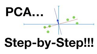
This video explains how to apply a Principal Component Analysis (PCA) in Python. More details: https://statisticsglobe.com/principal...

The video is presented by Cansu Kebabci, a data scientist and statistician at Statistics Globe. Find more information about Cansu here: https://statisticsglobe.com/cansu-keb...

In the video, Cansu explains the steps and application of a Principal Component Analysis in Python. Watch the video to learn more on this topic!

Here can you find the previous videos of this series:

Introduction to Principal Component Analysis (Pt. 1 - Theory):    • Introduction to Principal Component A...  

Principal Component Analysis in R Programming (Pt. 2 - PCA in R):    • Principal Component Analysis in R Pro...  

Links to the tutorials mentioned in the video:

PCA Using Correlation & Covariance Matrix (Examples): https://statisticsglobe.com/pca-corre...

Biplot for PCA Explained: https://statisticsglobe.com/biplot-pc...

Python code of this video:

Install libraries
!pip install scikit-learn
!pip install pandas
!pip install matplotlib
!pip install numpy

Load Libraries & Modules
import numpy as np
import pandas as pd
from sklearn.datasets import load_breast_cancer
from sklearn.decomposition import PCA
from sklearn.preprocessing import StandardScaler
import matplotlib.pyplot as plt

Load Breast Cancer Dataset
breast_cancer = load_breast_cancer()

Data Elements of breast_cancer
breast_cancer.keys()
breast_cancer.data.shape
breast_cancer.feature_names

Print Data in DataFrame Format
DF = pd.DataFrame(data = breast_cancer.data[:, :10], # Create DataFrame DF
columns = breast_cancer.feature_names[:10])
DF.head(6) # Print first 6 rows of DF

Standardize Data
scaler = StandardScaler() # Create scaler
data_scaled = scaler.fit_transform(DF) # Fit scaler
print(data_scaled) # Print scaler


Print Standardized Data in DataFrame Format
DF_scaled = pd.DataFrame(data = data_scaled,
columns = data.feature_names[:10])
DF_scaled.head(6)


Print Standardized Data in DataFrame Format
DF_scaled = pd.DataFrame(data = data_scaled, # Create DataFrame DF_scaled
columns = breast_cancer.feature_names[:10])
DF_scaled.head(6) # Print first 6 rows of DF_scaled

Ideal Number of Components
pca = PCA(n_components = 10) # Create PCA object forming 10 PCs
pca_trans = pca.fit_transform(DF_scaled) # Transform data
print(pca_trans) # Print transformed data
print(pca_trans.shape) # Print dimensions of transformed data


prop_var = pca.explained_variance_ratio_ # Extract proportion of explained variance
print(prop_var) # Print proportion of explained variance


PC_number = np.arange(pca.n_components_) + 1 # Enumarate component numbers
print(PC_number) # Print component numbers

Scree Plot
plt.figure(figsize=(10, 6)) # Set figure and size
plt.plot(PC_number, # Plot prop var
prop_var,
'ro-')
plt.title('Scree Plot (Elbow Method)', # Plot Annotations
fontsize = 15)
plt.xlabel('Component Number',
fontsize = 15)
plt.ylabel('Proportion of Variance',
fontsize = 15)
plt.grid() # Add grid lines
plt.show() # Print graph

#Alternative Scree Plot Data
var = pca.explained_variance_ # Extract explained variance
print(var) # Print explained variance

The remaining code is unfortunately too long for a YouTube description.

Follow me on Social Media:
Facebook – Statistics Globe Page:   / statisticsglobecom  
Facebook – R Programming Group for Discussions & Questions:   / statisticsglobe  
Facebook – Python Programming Group for Discussions & Questions:   / statisticsglobepython  
LinkedIn – Statistics Globe Page:   / statisticsglobe  
LinkedIn – R Programming Group for Discussions & Questions:   / 12555223  
LinkedIn – Python Programming Group for Discussions & Questions:   / 12673534  
Twitter:   / joachimschork  
Instagram:   / statisticsglobecom  
TikTok:   / statisticsglobe